
Has there ever been a time when you wish the day would never end?
Jenn, Founder Calcworkshop ® , 15+ Years Experience (Licensed & Certified Teacher)
Or, on the flip side, have you ever felt like the day couldn’t end fast enough?
What do these sentiments have in common?
Both are trying to optimize the situation!
Optimization is the process of finding maximum and minimum values given constraints using calculus.
For example, you’ll be given a situation where you’re asked to find:
It is our job to translate the problem or picture into usable functions to find the extreme values.
Step 1: Translate the problem using assign symbols, variables, and sketches, when applicable, by finding two equations: one is the primary equation that contains the variable we wish to optimize, and the other is called the secondary equation, which holds the constraints.
Step 2: Substitute our secondary equation into our primary equation and simplify.
Step 3: Take the first derivative of this simplified equation and set it equal to zero to find critical numbers.
Step 4: Verify our critical numbers yield the desired optimized result (i.e., maximum or minimum value).
While this may seem difficult at first, it’s really quite straightforward as we are simply finding two equations, plugging one equation into the other, and then taking the derivative.
Let’s look at a few problems to see how our optimization problem-solving strategies in work.
Suppose we are told that the product of two positive numbers is 192 and the sum is a minimum. What are the two numbers?
First, we need to find our primary and secondary equations by translating our problem.
Secondary: \(x \cdot y=192\)
Primary: \(x+y=\min\)
Now we will substitute our secondary equation into our primary equation (the equation we want to minimize) and simplify.
\begin
\text < If >x \cdot y=192 \rightarrow x=\frac, \text < then >x+y=\min \rightarrow \frac+y=\min
\end
Next, we will take the first derivative and solve for critical numbers by setting the derivative equal to zero.
Now, only the positive result fits our question because we are looking for two positive numbers. And now it’s time to use our second derivative test (or first derivative test) to verify that our critical number is indeed a relative minimum.
The second derivative is positive at the given critical number, so we know that we have a local minimum!
Now all that is left to do is substitute our found y-value into our original secondary equation to find the x-value.
Therefore, the two positive numbers whose product is 192 and sum is a minimum are \(x=\sqrt\) and \(y=\sqrt\).
See, that wasn’t too bad now, was it?
Okay, let’s now look at a more realistic question.
Assume the manager at a landscaping store wants to build a 600 square foot rectangular enclosure to display lawn equipment. Three sides of the enclosure will be made from wood fending at the cost of $7 per foot, whereas the fourth side of the enclosure will be built of bricks at the cost of $14 per foot. Find the dimensions of the least costly enclosure.
First, let’s draw a picture and find our primary and secondary equations.

Area Rectangular Enclosure
We know that the area of the enclosure is 600, so that would mean:
Now, we also know that three sides are wood, and one side is brick, so let’s relabel our diagram as follows.
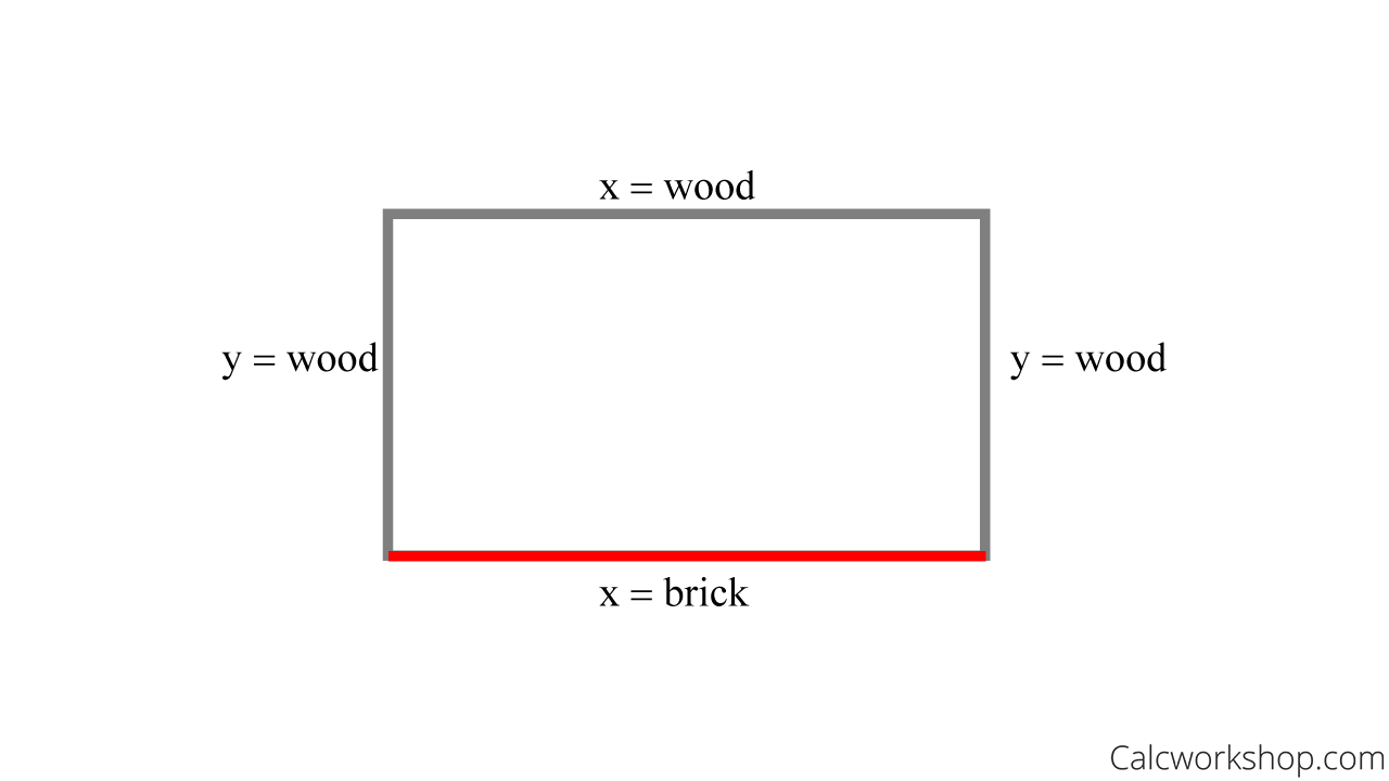
Cost Materials Rectangular Enclosure
And since the cost for the wood is $7 and brick is $14, that means the cost for the enclosure would be
Alright, so now we’ve acquired our two equations.
Primary: \(C=14 y+21 x\)
Secondary: \(x y=600\)
Now it’s time to substitute the secondary equation into the primary equation (the equation we want to optimize) and simplify
\begin
\begin
\text < If >x y=600 \rightarrow x=\frac=600 y^, \text < then >C=14 y+21 x \rightarrow C=14 y+21\left(600 y^\right) \\
C=14 y+12600 y^
\end
\end
Next, we will take the first derivative and solve for critical numbers by setting the derivative equal to zero.
Because the dimensions of an enclosure must be a positive distance, we know that the only critical number that makes sense is for y = 30 feet.
Now, let’s test our critical number, using the second derivative test, to ensure that this will yield a minimum value, as we are looking to find the least costly enclosure.
The second derivative is positive at y = 30, so we know that we have a local minimum!
Now all that is left to do is substitute our y-value into our secondary equation to find the x-value.
This means that the dimensions of the least costly enclosure are 20 feet long and 30 feet wide.
So, together we will work through numerous questions where we will have to follow the optimization problem-solving process to find the values that will either maximize or minimize our function.
Get access to all the courses and over 450 HD videos with your subscription
Monthly and Yearly Plans Available
Still wondering if CalcWorkshop is right for you?
Take a Tour and find out how a membership can take the struggle out of learning math.